Model
This page details the “quirks” of the model used for this website.
Predictions
This sections talks about the predictions made by the model.
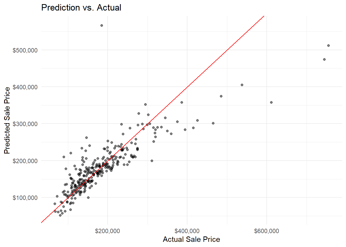
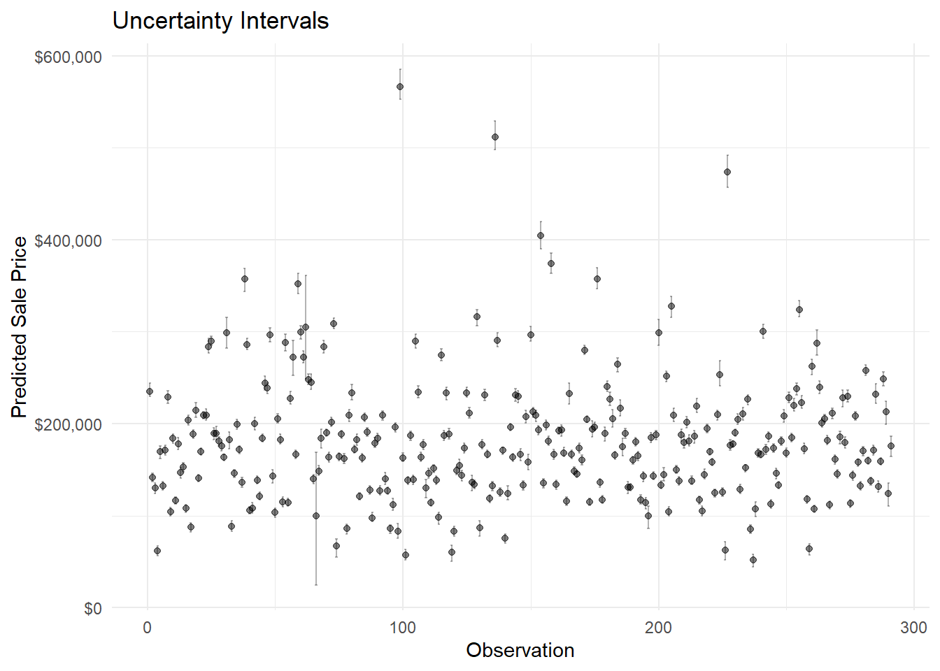
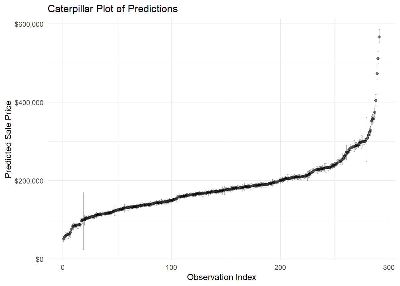
The predictions were created with the add_epred_draws() function from the tidybayes package. While still having some inaccuracy, this function is generally more accurate than its counterparts.
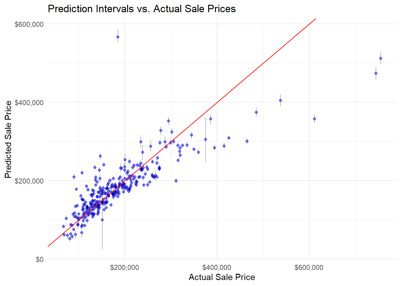
Here are some graphs detailing the predictions:
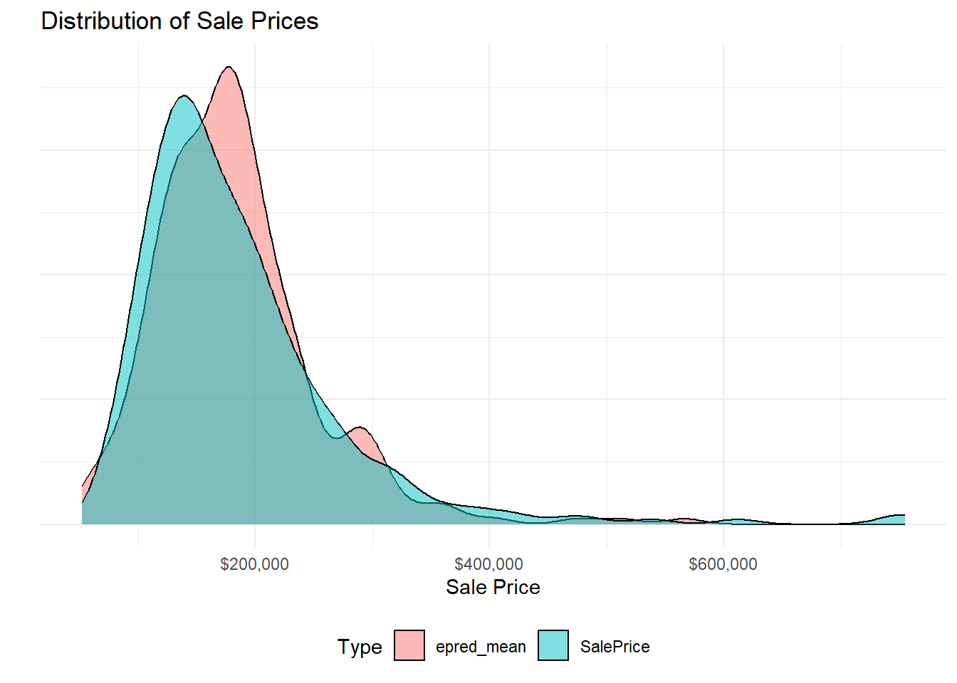
epred_mean is the predicted house prices.
Models
Model 1
This section talks about both models that are used in this website.
The first (and more accurate) model is a BRM model (Bayesian Regression Model). This is the model that is used for all of the graphs. The model uses a formula that includes all the variables in the data to predict how much each variable affects the total price of the house. The formula is \[ \begin{align*} \text{SalePrice} = \mathcal{N}(\mu_i, \sigma^2) \\ \mu_i = \beta_0 + \beta_1 \cdot \text{LotFrontage}_i + \beta_2 \cdot \text{LotArea}_i + \beta_3 \cdot \text{OverallQual}_i + \beta_4 \cdot \text{OverallCond}_i + \beta_5 \cdot \text{YearBuilt}_i + \beta_6 \cdot \text{YearRemodAdd}_i \\ + \beta_7 \cdot \text{MasVnrArea}_i + \beta_8 \cdot \text{BsmtFinSF1}_i + \beta_9 \cdot \text{BsmtFinSF2}_i + \beta_{10} \cdot \text{BsmtUnfSF}_i + \beta_{11} \cdot \text{TotalBsmtSF}_i \\ + \beta_{12} \cdot \text{X1stFlrSF}_i + \beta_{13} \cdot \text{X2ndFlrSF}_i + \beta_{14} \cdot \text{GrLivArea}_i + \beta_{15} \cdot \text{BsmtFullBath}_i + \beta_{16} \cdot \text{BsmtHalfBath}_i \\ + \beta_{17} \cdot \text{FullBath}_i + \beta_{18} \cdot \text{HalfBath}_i + \beta_{19} \cdot \text{BedroomAbvGr}_i + \beta_{20} \cdot \text{KitchenAbvGr}_i + \beta_{21} \cdot \text{TotRmsAbvGrd}_i \\ + \beta_{22} \cdot \text{Fireplaces}_i + \beta_{23} \cdot \text{GarageYrBlt}_i + \beta_{24} \cdot \text{GarageCars}_i + \beta_{25} \cdot \text{GarageArea}_i \\ + \beta_{26} \cdot \text{WoodDeckSF}_i + \beta_{27} \cdot \text{OpenPorchSF}_i + \beta_{28} \cdot \text{EnclosedPorch}_i + \beta_{29} \cdot \text{X3SsnPorch}_i + \beta_{30} \cdot \text{ScreenPorch}_i \\ + \beta_{31} \cdot \text{PoolArea}_i + \beta_{32} \cdot \text{MiscVal}_i \end{align*} \] Where:
\(\text{SalePrice}_i\) is the price of the house.
\(u_i\) is the linear predictor for the \(i\)-th house.
\(\beta_{0},\beta_{1},\beta_{2}...\beta_{32}\) are the coefficients.
\(\sigma^2\) is the variance of the Gaussian distribution.
Here’s a summary of the model:
Characteristic |
Beta |
95% CI 1 |
|---|---|---|
| LotFrontage | -0.81 | -20, 18 |
| LotArea | 0.24 | -0.01, 0.48 |
| OverallQual | 1.9 | -18, 22 |
| OverallCond | 0.21 | -19, 20 |
| YearBuilt | 32 | 13, 52 |
| YearRemodAdd | 24 | 3.4, 43 |
| MasVnrArea | 36 | 25, 48 |
| BsmtFinSF1 | 23 | 12, 34 |
| BsmtFinSF2 | -0.23 | -14, 13 |
| BsmtUnfSF | 10 | -1.1, 21 |
| TotalBsmtSF | 32 | 20, 44 |
| X1stFlrSF | 23 | 10, 36 |
| X2ndFlrSF | 27 | 16, 39 |
| GrLivArea | 40 | 29, 52 |
| BsmtFullBath | 0.08 | -19, 20 |
| BsmtHalfBath | 0.22 | -19, 20 |
| FullBath | 0.40 | -19, 21 |
| HalfBath | 0.16 | -19, 20 |
| BedroomAbvGr | -0.28 | -20, 19 |
| KitchenAbvGr | -0.21 | -21, 20 |
| TotRmsAbvGrd | 0.03 | -20, 20 |
| Fireplaces | 0.41 | -20, 21 |
| GarageYrBlt | 22 | 2.3, 41 |
| GarageCars | 0.43 | -20, 20 |
| GarageArea | 65 | 54, 76 |
| WoodDeckSF | 30 | 15, 44 |
| OpenPorchSF | 13 | -4.5, 30 |
| EnclosedPorch | -16 | -33, 1.2 |
| X3SsnPorch | 2.8 | -16, 22 |
| ScreenPorch | 9.2 | -8.2, 26 |
| PoolArea | -7.8 | -26, 11 |
| MiscVal | -1.3 | -5.8, 3.2 |
| 1
CI = Credible Interval |
||
And these are the values of the coefficients:
                   Estimate    Est.Error          Q2.5         Q97.5
Intercept     -1.583418e+05 3.304375e+04 -2.217716e+05 -9.187376e+04
LotFrontage   -8.130507e-01 9.750489e+00 -1.979193e+01  1.832144e+01
LotArea        2.369383e-01 1.256924e-01 -1.052083e-02  4.849382e-01
OverallQual    1.913311e+00 9.955828e+00 -1.829744e+01  2.212766e+01
OverallCond    2.098226e-01 9.838119e+00 -1.935090e+01  1.961939e+01
YearBuilt      3.191768e+01 9.919258e+00  1.252290e+01  5.170135e+01
YearRemodAdd   2.367911e+01 9.868182e+00  3.433188e+00  4.277861e+01
MasVnrArea     3.600668e+01 5.870588e+00  2.463411e+01  4.757421e+01
BsmtFinSF1     2.302873e+01 5.716336e+00  1.214155e+01  3.428110e+01
BsmtFinSF2    -2.302255e-01 6.823848e+00 -1.378719e+01  1.294171e+01
BsmtUnfSF      1.004742e+01 5.650464e+00 -1.085197e+00  2.089712e+01
TotalBsmtSF    3.215961e+01 6.041360e+00  2.040138e+01  4.405331e+01
X1stFlrSF      2.277109e+01 6.614810e+00  1.028781e+01  3.562506e+01
X2ndFlrSF      2.744346e+01 6.073054e+00  1.557852e+01  3.936512e+01
GrLivArea      4.015883e+01 6.032323e+00  2.852445e+01  5.188612e+01
BsmtFullBath   8.142487e-02 9.905329e+00 -1.885224e+01  1.956437e+01
BsmtHalfBath   2.163349e-01 9.898350e+00 -1.926754e+01  2.002975e+01
FullBath       3.964888e-01 1.031029e+01 -1.912795e+01  2.090468e+01
HalfBath       1.588439e-01 9.933301e+00 -1.911647e+01  1.957041e+01
BedroomAbvGr  -2.820032e-01 1.008818e+01 -2.005821e+01  1.930324e+01
KitchenAbvGr  -2.149270e-01 1.040331e+01 -2.086868e+01  1.975379e+01
TotRmsAbvGrd   2.708342e-02 1.009653e+01 -1.955919e+01  1.962530e+01
Fireplaces     4.105798e-01 1.017830e+01 -1.997695e+01  2.062880e+01
GarageYrBlt    2.151385e+01 9.930975e+00  2.256832e+00  4.090899e+01
GarageCars     4.308454e-01 1.010864e+01 -1.952893e+01  2.017322e+01
GarageArea     6.493535e+01 5.656480e+00  5.394206e+01  7.598057e+01
WoodDeckSF     2.965804e+01 7.309662e+00  1.513341e+01  4.416553e+01
OpenPorchSF    1.303416e+01 8.808714e+00 -4.490927e+00  2.965228e+01
EnclosedPorch -1.595668e+01 8.871181e+00 -3.325431e+01  1.244544e+00
X3SsnPorch     2.757090e+00 9.732680e+00 -1.624005e+01  2.190627e+01
ScreenPorch    9.165835e+00 8.905417e+00 -8.157776e+00  2.597299e+01
PoolArea      -7.777164e+00 9.509116e+00 -2.561103e+01  1.130821e+01
MiscVal       -1.341129e+00 2.287116e+00 -5.790779e+00  3.192435e+00
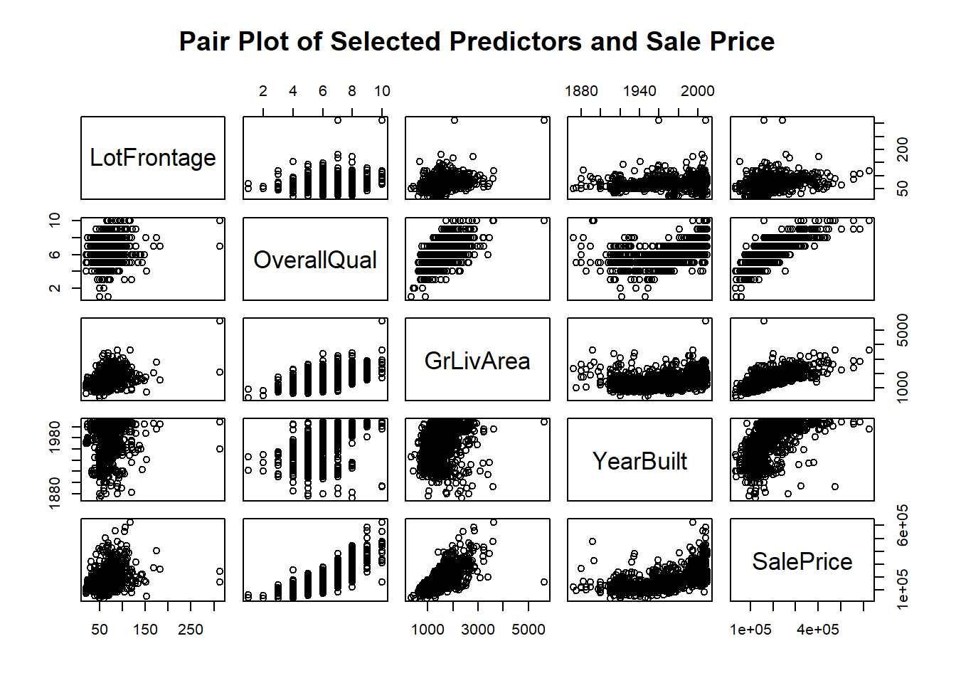
I’ve created a few graphs for this model, to show the “tech” stuff behind it.
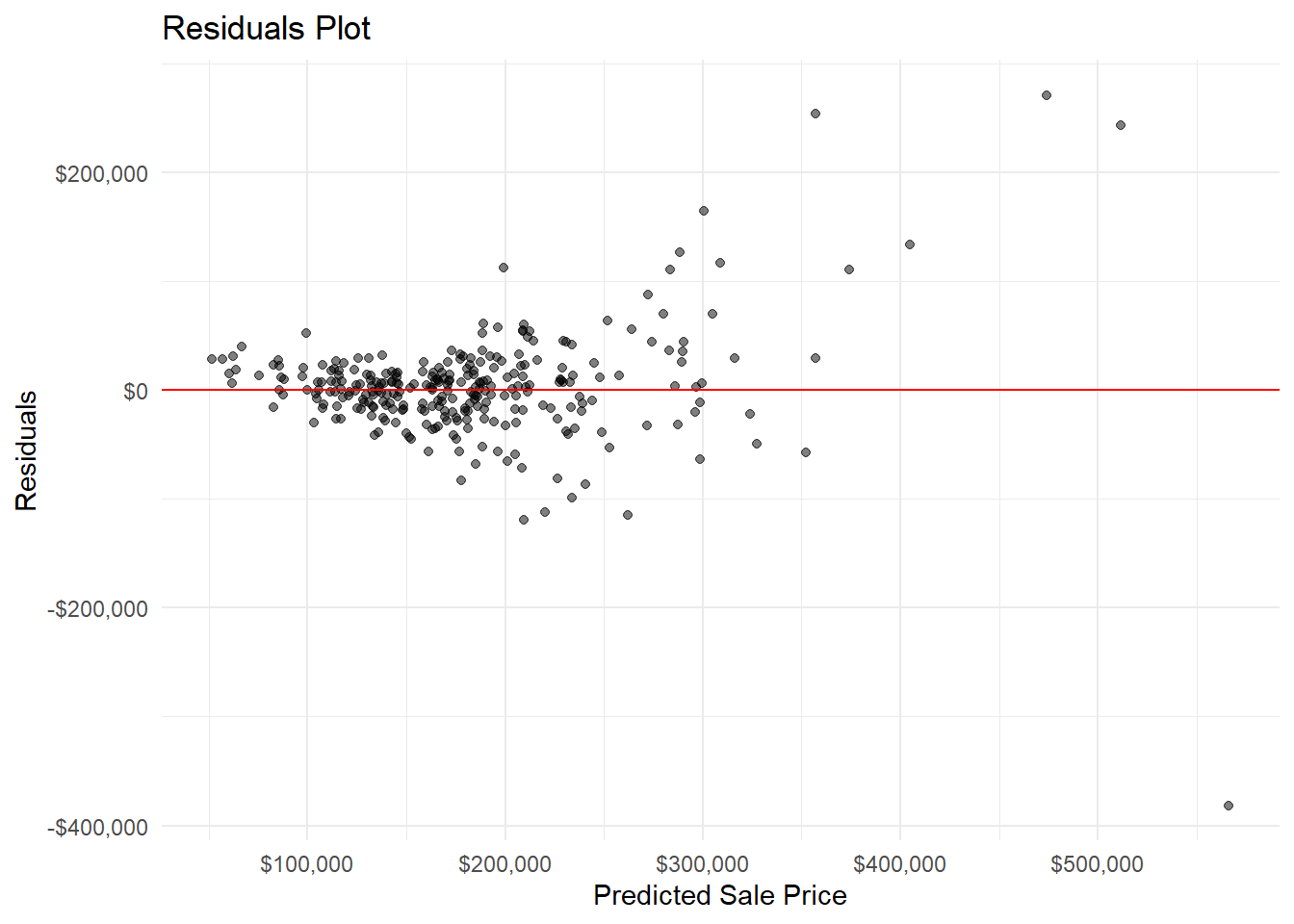
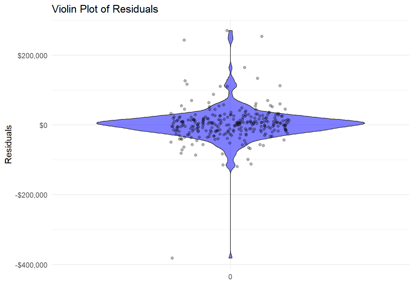
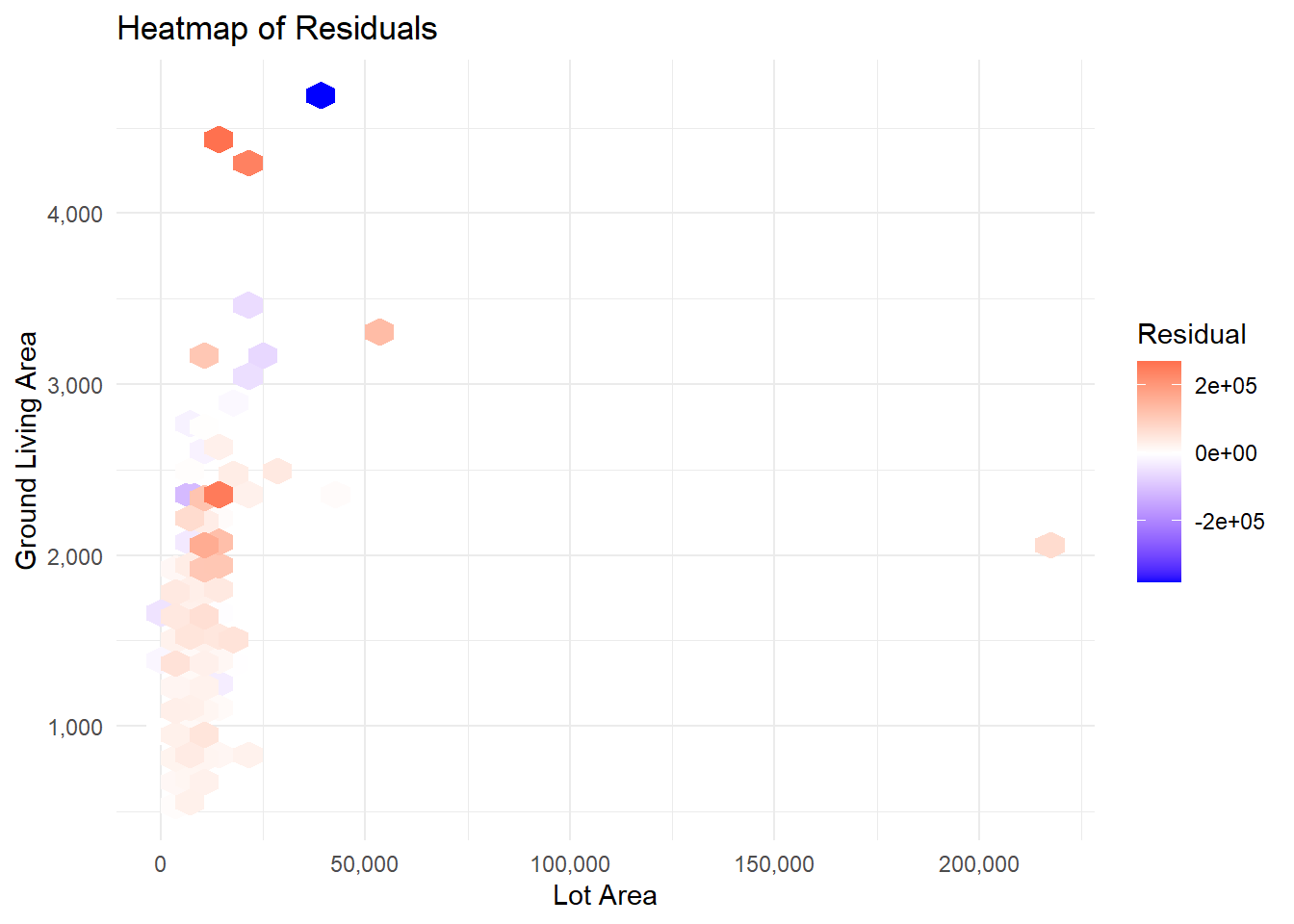
Residuals are the difference between predicted and actual values.
Model 2
The other (also BRM) model that was used was for only the House price estimator. This too was a BRM model, but it had fewer variables, thus making it less accurate. This was due to needing to simplify the model so the variables would be easier to type in (4 convenient inputs is much better than 32 estranged ones). However, the math is still the same pattern. Observe: \[ \begin{align*} \text{SalePrice}_i = \mathcal{N}(\mu_i, \sigma^2) \\ \mu_i = \beta_0 + \beta_1 \cdot \text{LotArea}_i + \beta_2 \cdot \text{OverallQual}_i + \beta_3 \cdot \text{GrLivArea}_i + \beta_4 \cdot \text{YearBuilt}_i \end{align*} \] Where:
\(\text{SalePrice}_i\) is the price of the house.
\(u_i\) is the linear predictor for the \(i\)-th house.
\(\beta_{0}...\beta_{4}\) are the coefficients.
\(\sigma^2\) is the variance of the Gaussian distribution.
Here’s a summary of the model:
Characteristic |
Beta |
95% CI 1 |
|---|---|---|
| LotArea | 0.77 | 0.48, 1.1 |
| OverallQual | 2.1 | -18, 22 |
| GrLivArea | 96 | 90, 101 |
| YearBuilt | 43 | 24, 62 |
| 1
CI = Credible Interval |
||
And these are the values of the coefficients:
                 Estimate    Est.Error          Q2.5         Q97.5
Intercept   -5.726317e+04 1.961196e+04 -9.456801e+04 -17781.804972
LotArea      7.741071e-01 1.503027e-01  4.767223e-01      1.060128
OverallQual  2.076136e+00 1.011661e+01 -1.777991e+01     21.996001
GrLivArea    9.554055e+01 2.727789e+00  9.023605e+01    100.788161
YearBuilt    4.322867e+01 9.724108e+00  2.411546e+01     61.841288